Output from KPP
This chapter describes the source code files that are generated by KPP.
The Fortran90 code
The code generated by KPP is organized in a set of separate files. Each
has a complete description of how it was generated at the begining of
the file. The files associated with root are named with a
corresponding prefix ROOT_ A short description of each file
is contained in the following sections.
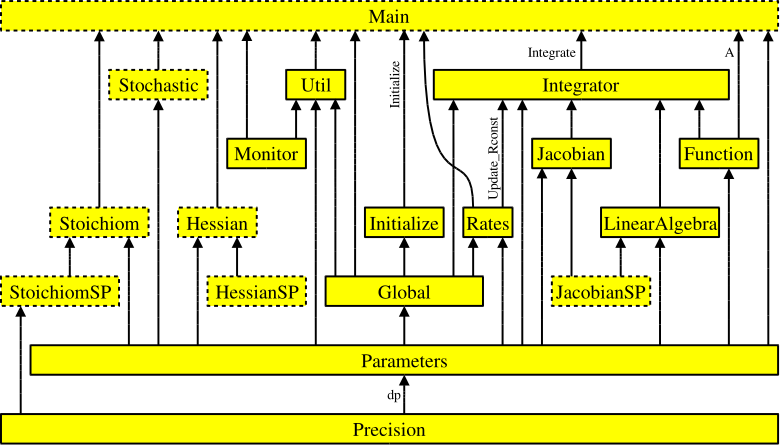
Figure 1: Interdependencies of the KPP-generated files. Each arrow
starts at the module that exports a variable or subroutine and
points to the module that imports it via the Fortran90 USE
instruction. The prefix ROOT_ has been omitted from module
names for better readability. Dotted boxes show optional files that
are only produced under certain circumstances.
All subroutines and functions, global parameters, variables, and
sparsity data structures are encapsulated in modules. There is exactly
one module in each file, and the name of the module is identical to the
file name but without the suffix .f90 or .F90. Figure 1
(above) shows how these modules are related to
each other. The generated code is consistent with the Fortran90
standard. It may, however, exceed the official maximum number of 39
continuation lines.
Tip
The default Fortran90 file suffix is .f90. To have KPP
generate Fortran90 code ending in .F90 instead, add the
command #UPPERCASEF90 ON to the KPP definition file.
ROOT_Main
ROOT_Main.f90 (or .F90) root is the main
Fortran90 program. It contains the driver after modifications by the
substitution preprocessor. The name of the file is computed by KPP by
appending the suffix to the root name.
Using #DRIVER none will skip generating this file.
ROOT_Model
The file ROOT_Model.f90 (or .F90) unifies all model
definitions in a single module. This simplifies inclusion into
external Fortran programs.
ROOT_Initialize
The file ROOT_Initialize.f90 (or .F9O)
contains the subroutine Initialize, which defines initial
values of the chemical species. The driver calls the subroutine once
before the time integration loop starts.
Note
In KPP 3.5.0 and later versions, you may pass the optional
PassiveSpc_ATOL_Threshold to subroutine Initialize
to prevent “passive” species intended for diagnostic purposes from
being used in certain computations (such as the Rosenbrock error
norm). At present this option is limited to Fortran90. For more
information, please see the Filtering out passive species with an absolute tolerance threshold section.
ROOT_Integrator
The file ROOT_Integrator.f90 (or .F90)
contains the subroutine Integrate, which is called every time
step during the integration. The integrator that was chosen with the
#INTEGRATOR command is also included in this file. In case
of an unsuccessful integration, the module root provides a short error
message in the public variable IERR_NAME.
ROOT_Monitor
The file ROOT_Monitor.f90 (.F90) contains
arrays with information about the chemical mechanism. The names of all
species are included in SPC_NAMES and the names of all
equations are included in EQN_NAMES.
It was shown (cf. #EQNTAGS) that each reaction in the section may start with an equation tag which is enclosed in angle brackets, e.g.:
<R1> NO2 + hv = NO + O3P : 6.69e-1*(SUN/60.0e0);
If the equation tags are switched on, KPP also generates the
PARAMETER array EQN_TAGS. In combination with
EQN_NAMES and the function tag2num that converts the
equation tag to the KPP-internal tag number, this can be used to
describe a reaction:
PRINT*, ’Reaction 1 is:’, EQN_NAMES( tag2num( ’R1’ ) )
ROOT_Precision
Fortran90 code uses parameterized real
types. ROOT_Precision.f90 (or .F90) contains the
following real kind definitions:
! KPP_SP - Single precision kind
  INTEGER, PARAMETER :: &
    SP = SELECTED_REAL_KIND(6,30)
! KPP_DP - Double precision kind
  INTEGER, PARAMETER :: &
    DP = SELECTED_REAL_KIND(12,300)
Depending on the choice of the #DOUBLE command, the real
variables are of type double (REAL(kind=dp)) or single
precision (REAL(kind=sp)). Changing the parameters of the
SELECTED_REAL_KIND function in this module will cause a change
in the working precision for the whole model.
ROOT_Rates
The code to update the rate constants is in ROOT_Rates.f90 (or
.F90). The user defined rate law functions (cf.
Fortran90 subrotutines in ROOT_Rates) are also placed here.
Function |
Description |
|---|---|
|
Update photolysis rate coefficients |
|
Update all rate coefficients |
|
Update sun intensity |
ROOT_Parameters
Global parameters are defined and initialized in
ROOT_Parameters.f90 (or .F90):
Parameter |
Represents |
Example |
|---|---|---|
|
No. chemical species ( |
7 |
|
No. variable species |
5 |
|
No. fixed species |
2 |
|
No. reactions |
10 |
|
No. nonzero entries Jacobian |
18 |
|
As above, after LU factorization |
19 |
|
Length, sparse Hessian |
10 |
|
Length, sparse Jacobian JVRP |
13 |
|
Length, stoichiometric matrix |
22 |
|
Index of species spc in |
|
|
Index of fixed species spc in |
Example values listed in the 3rd column are taken from the small_strato mechanism (cf. Running KPP with an example stratospheric mechanism).
KPP orders the variable species such that the sparsity pattern of the
Jacobian is maintained after an LU decomposition. For our example there
are five variable species (NVAR = 5) ordered as
ind_O1D=1, ind_O=2, ind_O3=3, ind_NO=4, ind_NO2=5
and two fixed species (NFIX = 2)
ind_M = 6, ind_O2 = 7.
KPP defines a complete set of simulation parameters, including the numbers of variable and fixed species, the number of chemical reactions, the number of nonzero entries in the sparse Jacobian and in the sparse Hessian, etc.
ROOT_Global
Several global variables are declared in ROOT_Global.f90 (or
.F90):
Global variable |
Represents |
|---|---|
|
Concentrations, all species |
|
Concentrations, variable species (pointer) |
|
Concentrations, fixed species (pointer) |
|
Rate coefficient values |
|
Current integration time |
|
Sun intensity between 0 and 1 |
|
Temperature |
|
Simulation start/end time |
|
Simulation time step |
|
Absolute tolerances |
|
Relative tolerances |
|
Lower bound for time step |
|
Upper bound for time step |
|
Conversion factor |
Both variable and fixed species are stored in the one-dimensional
array C. The first part (indices from 1 to NVAR)
contains the variable species, and the second part (indices from to
NVAR+1 to NSPEC) the fixed species. The total number
of species is the sum of the NVAR and NFIX. The parts
can also be accessed separately through pointer variables VAR and
FIX, which point to the proper elements in C.
VAR(1:NVAR) => C(1:NVAR)
FIX(1:NFIX) => C(NVAR+1:NSPEC)
Important
In previous versions of KPP, Fortran90 code was generated with
VAR and FIX being linked to the C array
with an EQUIVALENCE statement. This construction, however,
is not thread-safe, and it prevents KPP-generated Fortran90 code
from being used within parallel environments (e.g. such as an
OpenMP parallel loop).
We have modified KPP 2.5.0 and later versions to make KPP-generated
Fortran90 code thread-safe. VAR and
FIX are now POINTER variables that
point to the proper slices of the C array. They are also
nullified when no longer needed. VAR and FIX are
now also kept internal to the various integrator files located in
the $KPP_HOME/int directory.
ROOT_Function
The chemical ODE system for our small_strato example (described in Running KPP with an example stratospheric mechanism) is:
where square brackets denote concentrations of the species. The code for
the ODE function is in ROOT_Function.f90 (or .F90) The
chemical reaction mechanism represents a set of ordinary differential
equations (ODEs) of dimension . The concentrations of fixed species
are parameters in the derivative function. The subroutine computes
first the vector A of reaction rates and then the vector
Vdot of variable species time derivatives. The input arguments
V, F, RCT are the concentrations of variable
species, fixed species, and the rate coefficients,
respectively. A and Vdot may be returned to the
calling program (for diagnostic purposes) with optional ouptut
argument Aout. Below is the Fortran90
code generated by KPP for the ODE function of our
small_strato example.
SUBROUTINE Fun (V, F, RCT, Vdot, Aout, Vdotout )

! V - Concentrations of variable species (local)
  REAL(kind=dp) :: V(NVAR)
! F - Concentrations of fixed species (local)
  REAL(kind=dp) :: F(NVAR)
! RCT - Rate constants (local)
  REAL(kind=dp) :: RCT(NREACT)
! Vdot - Time derivative of variable species concentrations
  REAL(kind=dp) :: Vdot(NVAR)
! Aout - Optional argument to return equation rate constants
  REAL(kind=dp), OPTIONAL :: Aout(NREACT)


! Computation of equation rates
  A(1) = RCT(1)*F(2)
  A(2) = RCT(2)*V(2)*F(2)
  A(3) = RCT(3)*V(3)
  A(4) = RCT(4)*V(2)*V(3)
  A(5) = RCT(5)*V(3)
  A(6) = RCT(6)*V(1)*F(1)
  A(7) = RCT(7)*V(1)*V(3)
  A(8) = RCT(8)*V(3)*V(4)
  A(9) = RCT(9)*V(2)*V(5)
  A(10) = RCT(10)*V(5)

  !### Use Aout to return equation rates
  IF ( PRESENT( Aout ) ) Aout = A

! Aggregate function
  Vdot(1) = A(5)-A(6)-A(7)
  Vdot(2) = 2*A(1)-A(2)+A(3) &
            -A(4)+A(6)-A(9)+A(10)
  Vdot(3) = A(2)-A(3)-A(4)-A(5) &
            -A(7)-A(8)
  Vdot(4) = -A(8)+A(9)+A(10)
  Vdot(5) = A(8)-A(9)-A(10)

END SUBROUTINE Fun
ROOT_Jacobian and ROOT_JacobianSP
The Jacobian matrix for our example contains 18 non-zero elements:
It defines how the temporal change of each chemical species depends on
all other species. For example, \(\mathbf{J}(5,2)\) shows that \(NO_2\)
(species number 5) is affected by \(O\) (species number 2) via
reaction R9. The sparse data structures for the Jacobian are
declared and initialized in ROOT_JacobianSP.f90 (or
.F90). The code for the ODE Jacobian and
sparse multiplications is in ROOT_Jacobian.f90 (or
.F90).
Tip
Adding either #JACOBIAN SPARSE_ROW or
#JACOBIAN SPARSE_LU_ROW to the KPP definition file will
create the file ROOT_JacobianSP.f90 (or .F90).
The Jacobian of the ODE function is automatically constructed by KPP.
KPP generates the Jacobian subroutine Jac or JacSP where
the latter is generated when the sparse format is required. Using the
variable species V, the fixed species F, and the rate
coefficients RCT as input, the subroutine calculates the
Jacobian JVS. The default data structures for the sparse
compressed on rows Jacobian representation (for the case where the LU
fill-in is accounted for) are:
Global variable |
Represents |
|---|---|
|
Jacobian nonzero elements |
|
Row indices |
|
Column indices |
|
Start of rows |
|
Diagonal entries |
JVS stores the LU_NONZERO elements of the
Jacobian in row order. Each row I starts at position
LU_CROW(I), and LU_CROW(NVAR+1) =
LU_NONZERO+1. The location of the I-th diagonal
element is LU_DIAG(I). The sparse element JVS(K) is
the Jacobian entry in row LU_IROW(K) and column
LU_ICOL(K). For the small_strato example KPP
generates the following Jacobian sparse data structure:
LU_ICOL = (/ 1,3,1,2,3,5,1,2,3,4, &
            5,2,3,4,5,2,3,4,5 /)
LU_IROW = (/ 1,1,2,2,2,2,3,3,3,3, &
            3,4,4,4,4,5,5,5,5 /)
LU_CROW = (/ 1,3,7,12,16,20 /)
LU_DIAG = (/ 1,4,9,14,19,20 /)
This is visualized in Figure 2 below.. The sparsity coordinate vectors are computed by KPP and initialized statically. These vectors are constant as the sparsity pattern of the Jacobian does not change during the computation.
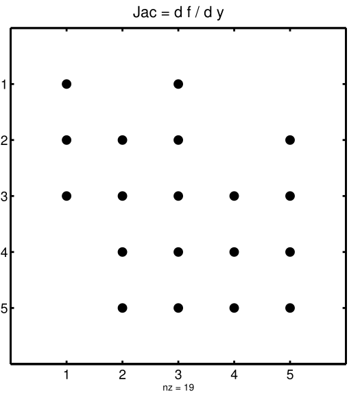
Figure 2: The sparsity pattern of the Jacobian for the small_strato example. All non-zero elements are marked with a bullet. Note that even though \(\mathbf{J}(3,5)\) is zero, it is also included here because of the fill-in.
Two other KPP-generated routines, Jac_SP_Vec and
JacTR_SP_Vec (see Fortran90 subroutines in ROOT_Jacobian) are useful for direct
and adjoint sensitivity analysis. They perform sparse multiplication of
JVS (or its transpose for JacTR_SP_Vec) with the
user-supplied vector UV without any indirect addressing.
Function |
Description |
|---|---|
|
ODE Jacobian in sparse format |
|
Sparse multiplication |
|
Sparse multiplication |
|
ODE Jacobian in full format |
ROOT_Hessian and ROOT_HessianSP
The sparse data structures for the Hessian are declared and initialized
in ROOT_Hessian.f90 (or .F90). The Hessian
function and associated sparse multiplications are in
ROOT_HessianSP.f90 (or .F90).
The Hessian contains the second order derivatives of the time derivative functions. More exactly, the Hessian is a 3-tensor such that
KPP generates the routine Hessian:
Function |
Description |
|---|---|
|
ODE Hessian in sparse format |
|
Hessian action on vectors |
|
Transposed Hessian action on vectors |
Using the variable species V, the fixed species F, and
the rate coefficients RCT as input, the subroutine
Hessian calculates the Hessian. The Hessian is a very sparse
tensor. The sparsity of the Hessian for our example is visualized in
Figure 3: The Hessian of the small_strato example.
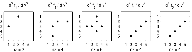
Figure 3: The Hessian of the small_strato example.
KPP computes the number of nonzero Hessian entries and saves it in the
variable NHESS. The Hessian itself is represented in
coordinate sparse format. The real vector HESS holds the values, and the
integer vectors IHESS_I, IHESS_J, and IHESS_K
hold the indices of nonzero entries as illustrated in Sparse Hessian Data.
Variable |
Represents |
|---|---|
|
Hessian nonzero elements \(H_{i,j,k}\) |
|
Index \(i\) of element \(H_{i,j,k}\) |
|
Index \(j\) of element \(H_{i,j,k}\) |
|
Index \(k\) of element \(H_{i,j,k}\) |
Since the time derivative function is smooth, these Hessian matrices
are symmetric, \(\tt HESS_{i,j,k}\)=\(\tt HESS_{i,k,j}\).
KPP stores only those entries \(\tt HESS_{i,j,k}\) with
\(j \le k\). The sparsity coordinate vectors IHESS_1,
IHESS_J and IHESS_K are computed by KPP and
initialized statically. They are constant as the sparsity pattern of
the Hessian does not change during the computation.
The routines Hess_Vec and HessTR_Vec compute the
action of the Hessian (or its transpose) on a pair of user-supplied
vectors U1 and U2. Sparse operations are employed to
produce the result vector.
ROOT_LinearAlgebra
Sparse linear algebra routines are in the file
ROOT_LinearAlgebra.f90 (or .F90). To
numerically solve for the chemical concentrations one must employ an
implicit timestepping technique, as the system is usually stiff. Implicit
integrators solve systems of the form
where the matrix \(P=I - h \gamma J\) is refered to as the “prediction matrix”. \(I\) the identity matrix, \(h\) the integration time step, \(\gamma\) a scalar parameter depending on the method, and \(J\) the system Jacobian. The vector \(b\) is the system right hand side and the solution \(x\) typically represents an increment to update the solution.
The chemical Jacobians are typically sparse, i.e. only a relatively small number of entries are nonzero. The sparsity structure of \(P\) is given by the sparsity structure of the Jacobian, and is produced by KPP (with account for the fill-in) as discussed above.
KPP generates the sparse linear algebra subroutine KppDecomp
(see Fortran90 functions in ROOT_LinearAlgebra) which performs an in-place, non-pivoting,
sparse LU decomposition of the prediction matrix \(P\). Since the
sparsity structure accounts for fill-in, all elements of the full LU
decomposition are actually stored. The output argument IER
returns a value that is nonzero if singularity is detected.
Function |
Description |
|---|---|
|
Sparse LU decomposition |
|
Sparse back substitution |
|
Transposed sparse back substitution |
The subroutines KppSolve and KppSolveTr and use the
in-place LU factorization \(P\) as computed by and perform sparse
backward and forward substitutions (using \(P\) or its
transpose). The sparse linear algebra routines KppDecomp and
KppSolve are extremely efficient, as shown by
Sandu et al. [1996].
ROOT_Stoichiom and ROOT_StoichiomSP
These files contain contain a description of the chemical mechanism in
stoichiometric form. The file ROOT_Stoichiom.f90 (or
.F90) contains the functions for reactant
products and its Jacobian, and derivatives with respect to rate
coefficients. The declaration and initialization of the stoichiometric
matrix and the associated sparse data structures is done in
ROOT_StochiomSP.f90 (or .F90).
Tip
Adding #STOICMAT ON to the KPP definition file will
create the file ROOT_Stoichiom.f90 (or .F90)
Also, if either #JACOBIAN SPARSE ROW or
#JACOBIAN SPARSE_LU_ROW are also added to the KPP
definition file, the file ROOT_StoichiomSP.f90 (or
.F90) will also be created.
The stoichiometric matrix is constant sparse. For our example the matrix
NSTOICM=22 has 22 nonzero entries out of 50 entries. KPP produces the
stoichiometric matrix in sparse, column-compressed format, as shown in
Sparse Stoichiometric Matrix. Elements are stored in columnwise order in the
one-dimensional vector of values STOICM. Their row and column indices
are stored in ICOL_STOICM and ICOL_STOICM
respectively. The vector CCOL_STOICM contains pointers to
the start of each column. For example column j starts in the sparse
vector at position CCOL_STOICM(j) and ends at
CCOL_STOICM(j+1)-1. The last value CCOL_STOICM(NVAR) =
NSTOICHM+1 simplifies the handling of sparse data structures.
Variable |
Represents |
|---|---|
|
Stoichiometric matrix |
|
Row indices |
|
Column indices |
|
Start of columns |
Variable |
Represents |
|---|---|
|
Derivatives of Fun w/r/t rate coefficients |
|
Derivatives of Jac w/r/t rate coefficients |
|
Reactant products |
|
Jacobian of reactant products |
The subroutine ReactantProd (see Fortran90 functions in ROOT_Stoichiom)
computes the reactant products ARP for each reaction, and the
subroutine JacReactantProd computes the Jacobian of reactant products
vector, i.e.:
The matrix JVRP is sparse and is computed and stored in row
compressed sparse format, as shown in Fortran90 functions in ROOT_Hessian. The
parameter NJVRP holds the number of nonzero elements. For our
small_strato example:
NJVRP = 13
CROW_JVRP = (/ 1,1,2,3,5,6,7,9,11,13,14 /)
ICOL_JVRP = (/ 2,3,2,3,3,1,1,3,3,4,2,5,4 /)
Variable |
Represents |
|---|---|
|
Nonzero elements of |
|
Column indices of |
|
Row indices of |
|
Start of rows in |
If #STOICMAT is set to ON, the stoichiometric formulation allows a direct computation of the derivatives with respect to rate coefficients.
The subroutine dFun_dRcoeff computes the partial derivative
DFDR of the ODE function with respect to a subset of
NCOEFF reaction coefficients, whose indices are specified in the array
Similarly one can obtain the partial derivative of the Jacobian with
respect to a subset of the rate coefficients. More exactly, KPP
generates the subroutine dJacR_dCoeff, which calculates
DJDR, the product of this partial derivative with a
user-supplied vector U:
ROOT_Stochastic
If the generation of stochastic functions is switched on (i.e. when
the command #STOCHASTIC ON is added to the KPP definition
file), KPP produces the file ROOT_Stochastic.f90 (or .F90),
with the following functions:
Propensity calculates the propensity vector. The propensity
function uses the number of molecules of variable (Nmlcv) and
fixed (Nmlcf) species, as well as the stochastic rate
coefficients (SCT) to calculate the vector of propensity rates
(Propensity). The propensity \(\tt Prop_j\) defines the
probability that the next reaction in the system is the \(j^{th}\)
reaction.
StochasticRates converts deterministic rates to
stochastic. The stochastic rate coefficients (SCT) are
obtained through a scaling of the deterministic rate
coefficients (RCT). The scaling depends on the Volume
of the reaction container and on the number of molecules which react.
MoleculeChange calculates changes in the number of
molecules. When the reaction with index IRCT takes place, the
number of molecules of species involved in that reaction changes. The
total number of molecules is updated by the function.
These functions are used by the Gillespie numerical integrators (direct
stochastic simulation algorithm). These integrators are provided in both
Fortran90 and C implementations (the template file name is
gillespie). Drivers for stochastic simulations are also
implemented (the template file name is general_stochastic.).
ROOT_Util
In addition to the chemical system description routines discussed above,
KPP generates several utility subroutines and functions in the file
ROOT_Util.f90 (or .F90).
Function |
Description |
|---|---|
|
Check mass balance for selected atoms |
|
Shuffle concentration vector |
|
Shuffle concentration vector |
|
Utility for #LOOKAT command |
|
Utility for #LOOKAT command |
|
Utility for #LOOKAT command |
|
Calculate reaction number from equation tag |
|
Choose |
The subroutines InitSaveData, SaveData, and
CloseSaveData can be used to print the concentration of the
species that were selected with #LOOKAT to the file
ROOT.dat (cf. #LOOKAT and #MONITOR).
ROOT_mex_Fun, ROOT_mex_Jac_SP, and ROOT_mex_Hessian
Mex is a Matlab extension. KPP generates the mex routines for the ODE function, Jacobian, and Hessian, for the target languages C, Fortran77, and Fortran90.
Tip
To generate Mex files, add the command #MEX ON to the KPP definition file.
After compilation (using Matlab’s mex compiler) the mex functions can be called instead of the corresponding Matlab m-functions. Since the calling syntaxes are identical, the user only has to insert the mex string within the corresponding function name. Replacing m-functions by mex-functions gives the same numerical results, but the computational time could be considerably smaller, especially for large kinetic systems.
If possible we recommend to build mex files using the C language, as Matlab offers most mex interface options for the C language. Moreover, Matlab distributions come with a native C compiler (lcc) for building executable functions from mex files. The mex files built using Fortran90 may require further platform-specific tuning of the mex compiler options.
The C code
Important
Some run-time options for C-language integrators (specified in the ICNTRL and RCNTRL arrays) do not exactly correspond to the Fortran90 run-time options. We will standardize run-time integrator options across all target languages in a future KPP release.
The driver file ROOT.c contains the main (driver) program and
numerical integrator functions, as well as declarations and
initializations of global variables.
The generated C code includes three header files which are
#include-d in other files as appropriate.
The global parameters (cf. Parameters Declared in ROOT_Parameters) are
#include-d in the header fileROOT_Parameters.hThe global variables (cf. Global Variables Declared in ROOT_Global) are extern-declared in
ROOT_Global.hand declared in the driver fileROOT.c.The header file
ROOT_Sparse.hcontains extern declarations of sparse data structures for the Jacobian (cf. Sparse Jacobian Data Structures),Hessian (cf. Sparse Hessian Data) and stoichiometric matrix (cf. Sparse Stoichiometric Matrix), and the Jacobian of reaction products (cf. Sparse Data for Jacobian of Reactant Products). The actual declarations of each datastructures is done in the corresponding files.
The code for the ODE function (see section ROOT_Function) is in
ROOT_Function.c. The code for the ODE Jacobian and sparse
multiplications (cf. ROOT_Jacobian and ROOT_JacobianSP) is in
ROOT_Jacobian.c, and the declaration and initialization of the
Jacobian sparse data structures is in the file
ROOT_JacobianSP.c. Similarly, the Hessian function and
associated sparse multiplications (cf. ROOT_Hessian and ROOT_HessianSP)
are in ROOT_Hessian.c, and the declaration and initialization
of Hessian sparse data structures are in ROOT_HessianSP.c.
The file ROOT_Stoichiom.c contains the functions for reactant
products and its Jacobian, and derivatives with respect to rate coefficients
(cf. ROOT_Stoichiom and ROOT_StoichiomSP) . The declaration and
initialization of the stoichiometric matrix and the associated sparse
data structures (cf. Sparse Stoichiometric Matrix) is done in ROOT_StoichiomSP.c.
Sparse linear algebra routines (cf. ROOT_LinearAlgebra) are
in the file ROOT_LinearAlgebra.c. The code to update the rate
constants and user defined code for rate laws is in ROOT_Rates.c.
Various utility and input/output functions (cf. ROOT_Util) are in
ROOT_Util.c and ROOT_Monitor.c.
Finally, mex gateway routines that allow the C implementation of the ODE
function, Jacobian, and Hessian to be called directly from Matlab
(cf. ROOT_mex_Fun, ROOT_mex_Jac_SP, and ROOT_mex_Hessian) are also generated (in the files
ROOT_mex_Fun.c, ROOT_mex_Jac_SP.c, and
ROOT_mex_Hessian.c).
The Matlab code
Important
Some run-time options for Matlab-language integrators (specified in the ICNTRL and RCNTRL arrays) do not exactly correspond to the Fortran90 run-time options. We will standardize run-time integrator options across all target languages in a future KPP release.
Matlab provides a high-level programming environment that allows algorithm development, numerical computations, and data analysis and visualization. The KPP-generated Matlab code allows for a rapid prototyping of chemical kinetic schemes, and for a convenient analysis and visualization of the results. Differences between different kinetic mechanisms can be easily understood. The Matlab code can be used to derive reference numerical solutions, which are then compared against the results obtained with user-supplied numerical techniques. KPP/Matlab can also be used to teach students fundamentals of chemical kinetics and chemical numerical simulations.
Each Matlab function has to reside in a separate m-file. Function calls
use the m-function-file names to reference the function. Consequently,
KPP generates one m-function-file for each of the functions discussed in
the sections entitled ROOT_Function ,
ROOT_Jacobian and ROOT_JacobianSP, ROOT_Hessian and ROOT_HessianSP,
ROOT_Stoichiom and ROOT_StoichiomSP, ROOT_Util. The names of the
m-function-files are the same as the names of the functions (prefixed
by the model name ROOT.
The variables of Parameters Declared in ROOT_Parameters are defined as Matlab global
variables and initialized in the file
ROOT_parameter_defs.m. The variables of Global Variables Declared in ROOT_Global are
declared as Matlab global variables in the file
ROOT_global_defs.m. They can be accessed from within each
Matlab function by using declarations of the variables of interest.
The sparse data structures for the Jacobian (cf. Sparse Jacobian Data Structures), the Hessian
(cf. Sparse Hessian Data), the stoichiometric matrix (cf. Sparse Stoichiometric Matrix),
and the Jacobian of reaction (see Sparse Data for Jacobian of Reactant Products) are declared as
Matlab global variables in the file
ROOT_Sparse_defs.m. They are initialized in separate m-files,
namely ROOT_JacobianSP.m, ROOT_HessianSP.m, and
ROOT_StoichiomSP.m respectively.
Two wrappers (ROOT_Fun_Chem.m and ROOT_Jac_SP_Chem.m) are
provided for interfacing the ODE function and the sparse ODE Jacobian
with Matlab’s suite of ODE integrators. Specifically, the syntax of
the wrapper calls matches the syntax required by Matlab’s integrators
like ode15s. Moreover, the Jacobian wrapper converts the sparse KPP
format into a Matlab sparse matrix.
Function |
Description |
|---|---|
|
Driver |
|
Global parameters |
|
Global variables |
|
Global sparsity data |
|
Template for ODE function |
|
ODE function |
|
Template for ODE Jacobian |
|
Jacobian in sparse format |
|
Sparsity data structures |
|
ODE Hessian in sparse format |
|
Sparsity data structures |
|
Hessian action on vectors |
|
Transposed Hessian action on vectors |
|
Derivatives of Fun and Jac w/r/t rate coefficients |
|
Sparse data |
|
Reactant products |
|
Jacobian of reactant products |
|
User-defined rate reaction laws |
|
Update photolysis rate coefficients |
|
Update all rate coefficients |
|
Update sola intensity |
|
Check mass balance for selected atoms |
|
Set initial values |
|
Shuffle concentration vector |
|
Shuffle concentration vector |
The Makefile
KPP produces a Makefile that allows for an easy compilation of all
KPP-generated source files. The file name is Makefile_ROOT. The
Makefile assumes that the selected driver contains the main program.
However, if no driver was selected (i.e. #DRIVER none), it is
necessary to add the name of the main program file manually to the
Makefile.
The log file
The log file ROOT.log contains a summary of all the functions,
subroutines and data structures defined in the code file, plus a
summary of the numbering and category of the species involved.
This file contains supplementary information for the user. Several statistics are listed here, like the total number equations, the total number of species, the number of variable and fixed species. Each species from the chemical mechanism is then listed followed by its type and numbering.
Furthermore it contains the complete list of all the functions generated in the target source file. For each function, a brief description of the computation performed is attached containing also the meaning of the input and output parameters.
Output from the Integrators (ISTATUS and RSTATUS)
In order to obtain more information about the integration, KPP provides
the arrays ISTATUS (integer) and RSTATUS (real). Each of
them is an array of 20 elements. Array elements not listed here are
currently not used. Details can be found in the comment lines of the
individual integrator files in $KPP_HOME/int/.
ISTATUS
ISTATUS |
1 |
2 |
3 |
4 |
5 |
6 |
7 |
8 |
9 |
|---|---|---|---|---|---|---|---|---|---|
beuler |
Y |
Y |
Y |
Y |
Y |
Y |
Y |
Y |
|
dvode |
|||||||||
exponential |
|||||||||
feuler |
|||||||||
gillespie |
|||||||||
lsode |
Y |
Y |
Y |
||||||
radau5 |
Y |
Y |
Y |
Y |
Y |
Y |
Y |
Y |
|
rosenbrock |
Y |
Y |
Y |
Y |
Y |
Y |
Y |
Y |
|
rosenbrock_adj |
Y |
Y |
Y |
Y |
Y |
Y |
Y |
Y |
|
rosenbrock_autoreduce |
Y |
Y |
Y |
Y |
Y |
Y |
Y |
Y |
|
rosenbrock_h211b_qssa |
Y |
Y |
Y |
Y |
Y |
Y |
Y |
Y |
|
rosenbrock_tlm |
Y |
Y |
Y |
Y |
Y |
Y |
Y |
Y |
Y |
runge_kutta |
Y |
Y |
Y |
Y |
Y |
Y |
Y |
Y |
|
runge_kutta_adj |
Y |
Y |
Y |
Y |
Y |
Y |
Y |
Y |
|
runge_kutta_tlm |
Y |
Y |
Y |
Y |
Y |
Y |
Y |
Y |
|
sdirk |
Y |
Y |
Y |
Y |
Y |
Y |
Y |
Y |
|
sdirk_adj |
Y |
Y |
Y |
Y |
Y |
Y |
Y |
Y |
|
sdirk_tlm |
Y |
Y |
Y |
Y |
Y |
Y |
Y |
Y |
|
sdirk4 |
Y |
Y |
Y |
Y |
Y |
Y |
Y |
Y |
|
seulex |
Y |
Y |
Y |
Y |
Y |
Y |
Y |
||
tau_leap |
ISTATUS(1)
Number of times that the function containing the chemical ODE system was called.
ISTATUS(2)
Number times the Jacobian matrix was constructed.
ISTATUS(3)
Total number of integration timesteps.
ISTATUS(4)
Number of accepted timesteps.
ISTATUS(5)
Number of rejected timesteps (except at very beginning).
ISTATUS(6)
Number of LU decompositions that were performed.
ISTATUS(7)
Number of forward/backward substitutions that were performed.
ISTATUS(8)
Number of singular matrix decompositions that were performed.
ISTATUS(9)
Number of times the Hessian matrix was evaluated.
ISTATUS(10) .. ISTATUS(20)
Currently not used.
RSTATUS
RSTATUS |
1 |
2 |
3 |
4 |
|---|---|---|---|---|
beuler |
Y |
Y |
Y |
|
dvode |
||||
exponential |
||||
feuler |
Y |
|||
gillespie |
||||
lsode |
Y |
Y |
||
radau5 |
||||
rosenbrock |
Y |
Y |
Y |
|
rosenbrock_adj |
Y |
Y |
Y |
|
rosenbrock_autoreduce |
Y |
Y |
Y |
s |
rosenbrock_h211b_qssa |
Y |
Y |
Y |
|
rosenbrock_tlm |
Y |
Y |
Y |
|
runge_kutta |
Y |
Y |
Y |
|
runge_kutta_adj |
Y |
Y |
Y |
|
runge_kutta_tlm |
Y |
Y |
Y |
|
sdirk |
Y |
Y |
Y |
|
sdirk_adj |
Y |
Y |
Y |
|
sdirk_tlm |
Y |
Y |
Y |
|
sdirk4 |
Y |
Y |
||
seulex |
||||
tau_leap |
RSTATUS(1)
Texit, the time corresponding to the computed \(Y\)
upon return.
RSTATUS(2)
Hexit: the last accepted step before exit.
RSTATUS(3)
Hnew: The last predicted step (not yet taken. For multiple
restarts, use Hnew as Hstart in the subsequent run.
RSTATUS(4)
(Solver-specific for rosenbrock_autoreduce) AR_thr:
used to output the calculated (used) auto-reduction threshold for
the integration. Useful when ICNTRL(10) > 0 where the
threshold is dynamically determined based on a given species.
RSTATUS(5) .. RSTATUS(20)
Currently not used.